Basic statistics can easily be obtained for differnt parts of the image using this menu option. The user picks which of the following method to use to select the region of interest.
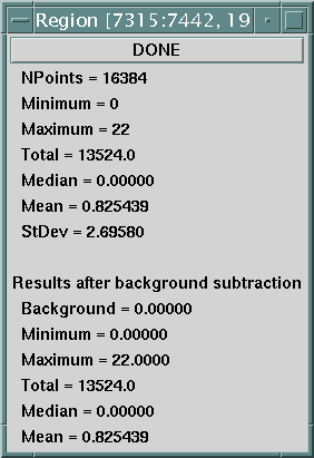
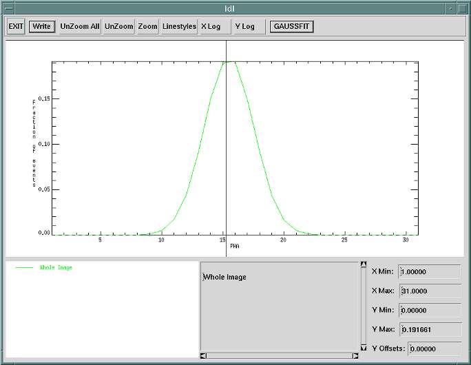
In the case of PHA statistics, a plot of the distribution of the Pulse Height is shown for either the whole image or the selected region.
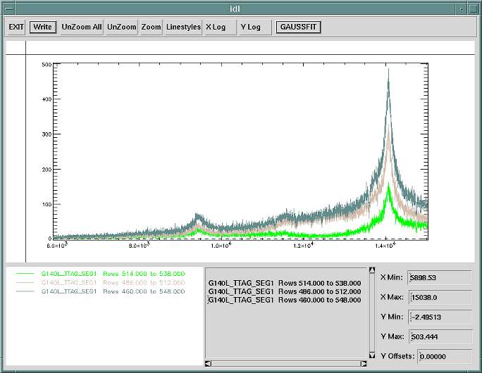
Many different plots can be generated with this menu option to examine the data closely. The width (in pixels) of the plot will be determined by the display WINDOW into which the cursor was located when the mouse button was clicked. Clicking in the Full Extend window will plot the whole width or height of the image. Clicking in the Main Window or the Zoomed Window will limit the extend of the plot to the region of the data displayed in that particular window.
It is possible for the user to display more than one row or column at a time in the plot window. By keeping the plot window on the screen and selecting multiple rows or columns one at a time, they are simply added to the plot window.
The plot window displays the multiple plots selected. The user can zoom in an area of the plot, change the axis to a logarithmic scale, change the type of lines used to trace each plot, write out the plots to a file as a Postscript plot, as an ASCII or FITS table or to a log file.
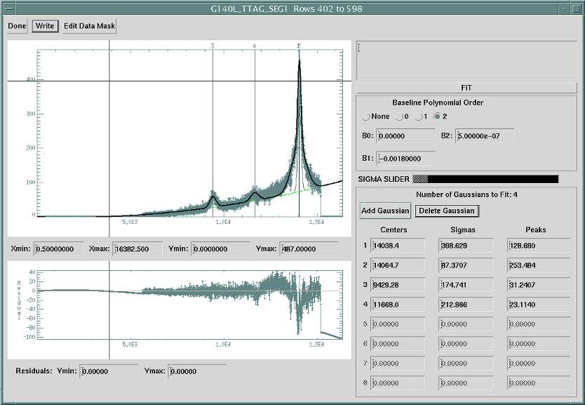
The user can also get a quick estimate the spectral line profile using the GAUSSFIT option with different type of baselines (none, constant or linear). For more elaborate Gaussian fits, the Interactive GaussFit Tool can be used.
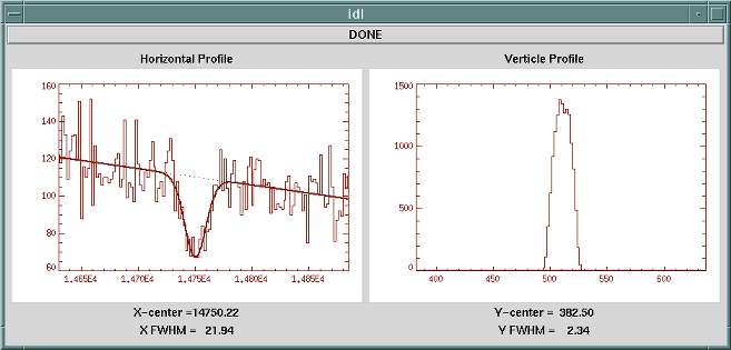
This menu option will calculate the best fit Gaussian in both X and Y for the data currently displayed in the Zoom Window. The data is coadded in X for the Vertical Profile and coadded in Y for the Horizontal Profile. The Center and Full Width at Half Maximum for each of the Gaussian is shown in the plot window with the data and the fitted curve.
The Time Tag menu option allows the user to view and/or edit the data currently loaded by selecting or removing data according to the time stamp information associated with every event recorded. Of course this tool is only available if the type of data loaded has this time stamp information available (observation done in TimeTag mode and not in ACCUM mode).
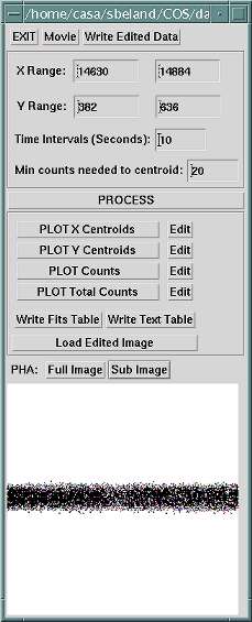
The user can select the region of interest to view/edit by typing in the desired XRange and YRange values (defaults to the Zoom window area). The time interval can also be selected (width of the bin in seconds) as well as the minimum number of counts in each time interval required to estimate the center of the data in X and Y. Once these parameters are acceptable, the data can be processed. The tool will go through the data and calculate the centroid pixel value for each time interval as well as the number of counts per time interval for the region of interest and for the whole image. This data can be written out as a FITS or an ASCII table.
The plot of the centroid allows the user to verify that the spectrum has not shifted in either direction on the detector during the observation. If any motion is detected, this data can be edited out by clicking on the Edit button corresponding to the specific plot. The tool that pops up is used to select a region of the data to ignore during further processing.
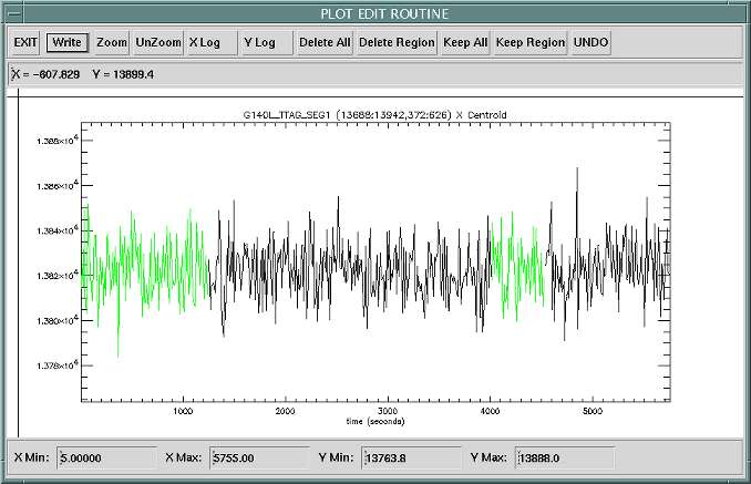
Once all the "correct" data has been selected (data within the specified time ranges have been removed), the user can then display the resulting image with the option i "Load Edited Image". This new data can also be saved as a FITS file with the "Write Edited Data" button.
It is possible to create a movie of the data as the events were recorded for the region of interest currently loaded (and possibly edited).
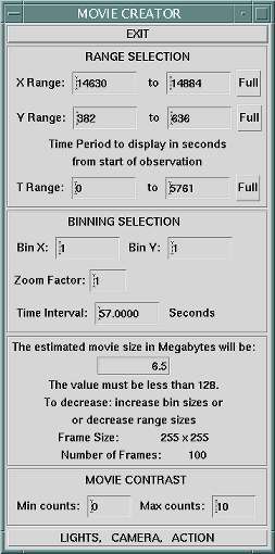
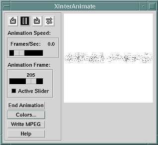
The user can select a different region than the one already chosen and restrict the time range to subset of the whole duration of the observation if desired. The data can also optionally be binned in X and/or Y and a different time interval can be chosen. By default a time interval is provided to get about 100 frames for the animation. The tool calculates the amount of memory needed to create the data array for the animation. Default contrast values are offered to the user. To view every single event, a value of 1 for the "Max counts:" should be selected. Once all the parameters have been selected, the user can then start the movie.
The animation frames will be created and loaded in memory for the first loop. Once all the frames are loaded, the animation starts. The user can control the speed, pause, stop or step through the animation and adjust or change the color table. The user can also save the animation to a file as an MPEG movie.